Materials and methods
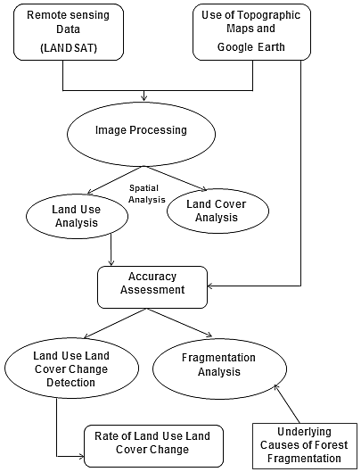
The procedure that we have followed in our present study is shown in Fig 2.
Fig 2: Flow chart of methodology followed in the study.
5.1. Pre-processing
The remote sensing data is processed to get the good insight into land use land cover analysis. The pre-processing of remote sensing data includes atmospheric correction and geometric correction inorder to enable correct area measurements, precise localization and multi-source data integration. The data obtained was geo-referenced with WGS-84 datum, rectified and cropped pertaining to the study area using Uttar Kannada boundary layer. The band correction was made using GRASS GIS (http://grass.osgeo.org/) in order to get the better and accurate results. The bands namely band-2 (Green), band-3 (Red) and band-4 (Near infrared) were used to produce the FCC (False Colour Composite). Google earth data was used for classification and validation.
5.2. Land Cover analysis
The normalized difference vegetation index (NDVI) is computed at temporal scale to determine the status of vegetation in Uttar Kannada. Among all techniques of land cover mapping NDVI is most widely accepted and applied. NDVI is calculated by using visible Red and NIR bands of Landsat data. The basic principle behind determining NDVI is that healthy vegetation absorbs most of the visible light that falls on it, and reflects a large portion of the near-infrared light however sparse vegetation reflects more visible light and less near-infrared light. NDVI for a given pixel always results in a number that ranges from minus one to plus one (-1 to +1). NDVI was calculated using the following equation;
NDVI = (NIR-R) / (NIR+R)
5.3. Land use analysis
The false colour composite image was generated to identify distinct patches in landscape. The temporal Remote Sensing data was used for classification. The classification is based on the assumption that each land use class reflects different amount of light and in different spectral region, the properties of which are also prominent in the remotely sensed data. The land use categories used in our study are; forest (which includes evergreen, semi-evergreen, moist deciduous, dry deciduous, scrub forests-grassland and forest plantations) and non-forest (which includes built up, cropland, open land and horticultural plantations like areca-coconut plantation). Supervised classification approach was used in which the signatures/sample areas of each forest and non-forest category/land use type are taken separately from the regions clearly attributable to any of the category. These samples are called training areas. This was made possible by using the digitized topographic map layers and Google earth by which the exact signature/sample of each category can be taken. The spectral information in all spectral bands for the pixels comprising these training areas is used to recognise spectrally similar areas for each class. Thus, in a supervised classification we are first identifying the information classes, which are then used to determine the spectral classes, which represent them.
Gaussian Maximum Likelihood decision rule was used to assign an unknown pixel to its respective land use class. The maximum likelihood classifier quantitatively evaluates both the variance and covariance of the category spectral response patterns while classifying an unknown pixel. It calculates the probability of each and every pixel in the image and after evaluating the probability in each category, the pixel would be assigned to the most likely class (highest probability value) or labelled "unknown" if the probability values are all below a threshold set by the analyst.
5.4. Accuracy Assessment
Accuracy assessment evaluates the performance of classifiers. Accuracy assessment and Kappa coefficient are common measurements used to demonstrate the effectiveness of the classifications (Congalton, 1991). The inaccuracies in spectral classification are measured by a set of reference pixels. Based on the reference pixels, confusion/error matrix (also called contingency table) is generated. Error matrices compare, on a category-by category basis, the relationship between known reference data (ground truth) and the corresponding results of an automated classification. Such matrices are square, with the number of rows and columns equal to the number of categories whose classification accuracy is being assessed. From the error matrices kappa (κ) statistics, overall accuracy and producer's and user's accuracies are computed, which determine how far our classification is accurate (Lillesand & Kiefer, 2004). Overall Accuracy = (Total number of correct pixels/ Total number of observed pixels) *100
User Accuracy = (Correct pixels/row total)*100
Producer accuracy = (Correct pixels/column total)*100
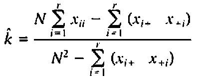
Where,
N = Total number of observations
r = Number of rows in matrix
Xii = Number of observations in row i and column i
Xi+ = Total number of observations in row i
X+i = Total number of observations in column i
5.5. Rate of Land use Change
The classified maps were analysed to identify the magnitude and direction of change. The compound interest formula due to its explicit biological meaning was used to assess the magnitude of the changes of various classes. It provided changes in the native land use/land cover category.
Change rate = {[Ln (At1)-Ln (At0)]/(t1-t0)}*100
Where At1 is area of class in current year, At0 is area of class in base year, t1 is current year, t0 is base year and Ln is natural logarithm.
5.5. Fragmentation Analysis.
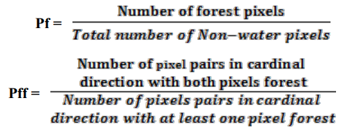
Forest fragmentation is the process whereby a large, continuous area of forest is both reduced in area and divided into two or more fragments. Fragmentation increases the number of habitat patches and decreases patch size. Sometimes, each habitat patch will be too small to sustain a local population. Species that are unable to cross the matrix will be then restricted to too small patches, reducing population sizes and the probability of their existence (Giulio et al., 2009). The decrease in the forest area and the increasing isolation between the forest patches has been the major cause of biodiversity loss.
In fragmentation analysis six fragmentation classes were considered which are; Interior (Pf=1), Patch (Pf<0.4), Transitional (0.4<Pf<0.6), Edge (Pf>0.6 and Pf-Pff>0), Perforated (Pf>0.6 and Pf-Pff<0) and Undetermined (Pf > 0.6 and Pf = Pff) where Pf is the proportion of pixels in the window that are forested and Pff is the proportion of all adjacent (cardinal directions only) pixel pairs that include at least one forest pixel, for which both pixels are forested. When Pff is larger than Pf, the implication is that forest is clumped; the probability that an immediate neighbour is also forest is greater than the average probability of forest within the window. Conversely, when Pff is smaller than Pf, the implication is that whatever is non-forest is clumped.